This Darchive is a reposting of this article from KIPAC research highlights: https://kipac.stanford.edu/highlights/confronting-models-des-year-3-data-or-how-did-we-get-here-and-whats-next
This article is based on the work in https://arxiv.org/abs/2105.13549 among many other papers. All the Year 3 analysis papers can be found on this page.
In the field of cosmology, and in Dark Energy Survey (DES) cosmology analyses more specifically, we aim to answer big questions like, “What is the Universe made of?”, “What does the large-scale Universe look like now and how has it changed over time?”, and “What forces govern that evolution?”
In the previous two posts about DES science, Justin Myles told you about how we’ve used galaxy colors to measure the distance to hundreds of millions of galaxies, and Jamie McCullough described how we can use the apparent shapes of those galaxies to map the distribution of matter in the Universe.
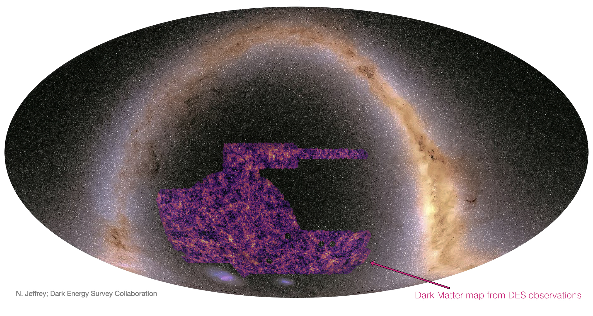
Figure 1: The Dark Energy Survey footprint displayed as a map of dark matter set against the entirety of the night sky above the Victor M. Blanco Telescope, located in the foothills of the Chilean Andes. (Credit: N. Jeffrey; DES Collaboration.)
These measurements are interesting not only because they allow us to make that map, but because of what they can tell us about the fundamental physics that has shaped the properties and history of the Universe. In this blog post, we’ll describe how we can go from the DES measurements of galaxy shapes and distances to constraints on fundamental physics, and thus to work towards answering the big open questions of cosmology.
Taking the measure of the Universe
In DES cosmology analyses we ultimately learn about physics by comparing the predictions of a model to measurements. Even with our most sophisticated models of the Universe, we can’t predict exactly where a given galaxy or clump of matter that is causing gravitational lensing will appear. However, we don’t need to do that to learn about physics! We just need to focus on something we can predict: the statistical properties of how we expect galaxy positions and the shear signal of weak gravitational lensing to be distributed relative to one another.
This means that when we compare our model to measurements, we’re not comparing models and measurements at the level of the full map of the positions and shapes of all the galaxies measured by DES. Instead we summarize information in those maps using statistical measurements. The statistical quantities used in our main DES galaxy clustering and weak lensing analysis are called “two-point correlation angular functions,” sometimes called two-point functions or just correlation functions for short.
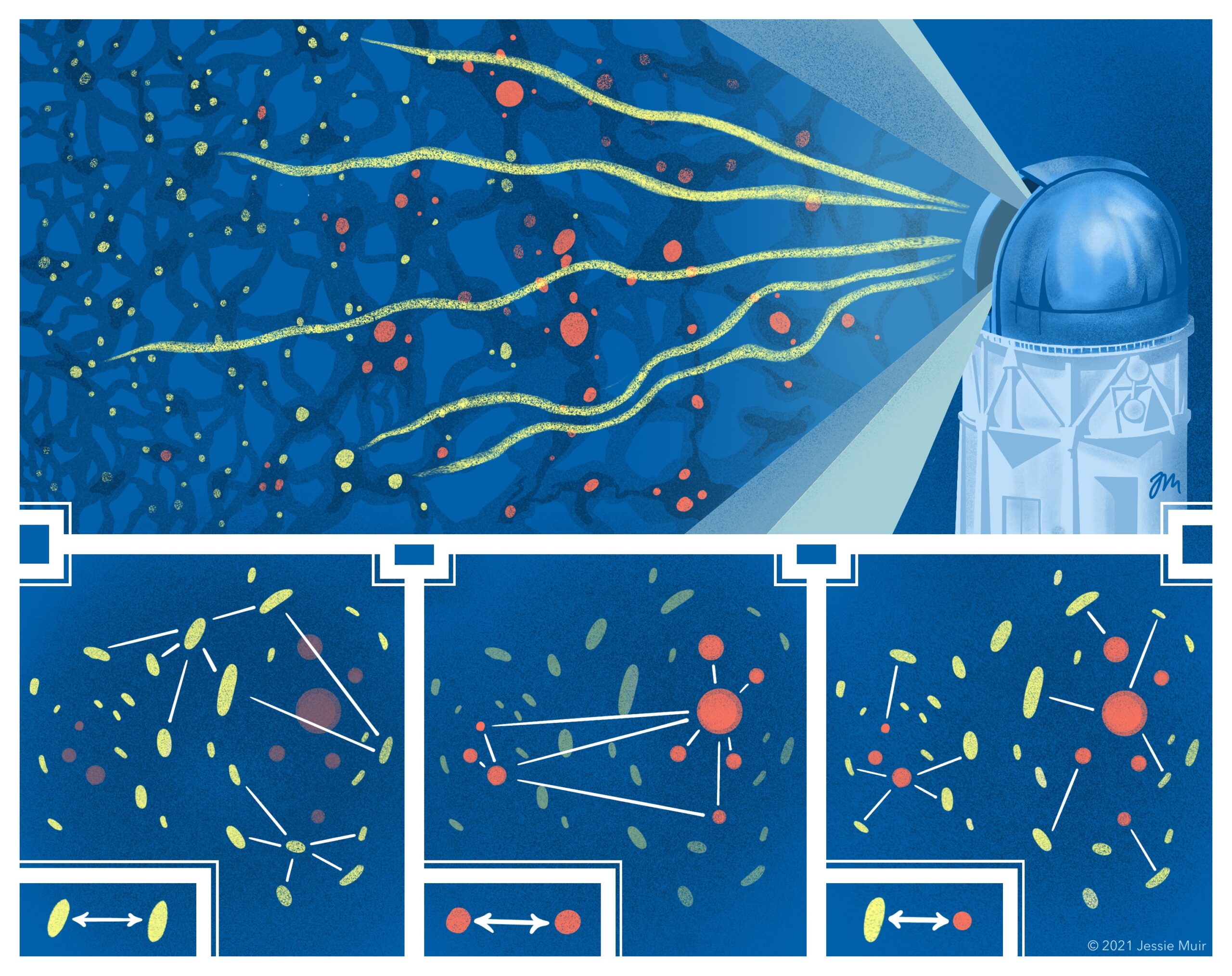
Figure 2: The three separate two-point correlations used by DES scientists to map the distribution of matter in the Universe. The DES analysis uses shape measurements of source galaxies, shown in yellow, and the positions of lens galaxies, shown in red. Bottom row, left to right: shear-shear correlations, galaxy-galaxy correlations, and galaxy-shear correlations (explained below). (Credit: Jessie Muir.)
A two-point angular correlation function describes the relationship between two kinds of measurements. For example, the correlation between galaxy positions tells you the probability of finding two galaxies with a given angular separation on the sky, relative to the probability you’d find if they were distributed randomly. Because gravity causes matter to clump over time, and galaxies trace these clumps, called overdensities, where matter has collected, we expect (and find!) galaxies to become more clustered over time. This information is captured in the galaxy-galaxy two-point correlation function.
We can similarly define a shear-shear two-point correlation function to describe weak lensing measurements: we expect more of that alignment between the shapes of galaxies which appear close to each other on the sky, because galaxies which are close to each other are more likely to be lensed by similar structures along the line of sight.
We also look at the correlation between weak lensing shear and the positions of galaxies that reside in the structures acting as lenses (the galaxy-shear two-point correlation function). Source galaxy shapes are distorted by lensing in a tangential pattern around overdensities, in the same way that images near the edge of a magnifying glass get distorted in a ring pattern. Since the lens galaxy positions trace the positions of those overdensities, looking at the alignment between (background) source galaxy shapes and (foreground) lens galaxy positions provides additional information about the distribution of dark matter.
We use this collection of two-point correlation functions—galaxy-galaxy, shear-shear, and galaxy-shear—to compare DES measurements to predictions from our cosmological model.
A model Universe
What ingredients are needed to make predictions for these quantities? One important piece of this puzzle is our theory of gravity, General Relativity. Gravity causes mass to attract mass, so describing that attraction is a key part of understanding how matter clumps up over time. It enables us to describe the transition from an early Universe that is nearly uniform with small fluctuations in density (whose initial properties are part of the inputs to our model), to the present, where non-uniformities have grown enough to create galaxies and planets and science bloggers.
This theory of gravity also allows us to describe the overall expansion of the Universe. General Relativity relates the behavior of space-time to the matter and energy in it. Given a description of how much of the Universe is made of dark matter, how much is baryonic (ordinary) matter, and how much is dark energy, we can describe how the Universe expands over time. That expansion influences the clustering of matter in the Universe because more rapid expansion will make it harder for matter to fall into overdensities, thus slowing the formation of structure. Expansion also affects the geometry related to how we measure distances to galaxies, and thus the relationship between the physical length scales of cosmological structures to how large they appear on the sky, as well as how they contribute to gravitational lensing.
Given these ingredients we can specify our cosmological model—that is, our description of the Universe’s expansion history and how structures within it grow—by choosing values for a set of parameters describing properties like the amplitude of density fluctuations and average density of matter in the Universe. In the main DES Year 3 galaxy clustering and weak lensing analysis, we vary 31 parameters: six characterizing the cosmological model, and 25 describing astrophysical effects and measurement uncertainties that must be accounted for to relate the cosmological physics to our observations. For any choice of values for these 31 parameters, we can make a prediction for the two-point correlation functions that we would expect to observe.
Where the measurement meets the model
The next step is to compare those model predictions to our actual two-point correlation function measurements, and to use that comparison to learn about physics. We strategically sample different values of our model parameters—for example, matter density, Ωm—and look at what parameter values produce a better or worse fit to the data. Based on how that goodness-of-fit changes when we vary parameters, we estimate a statistical quantity called the posterior. The posterior describes the probability, based on our observations, that a given set of parameter values are the true description of the physics of the Universe. We use the posterior probability to estimate parameter values and their uncertainties, using plots like that shown in Figure 3, below.
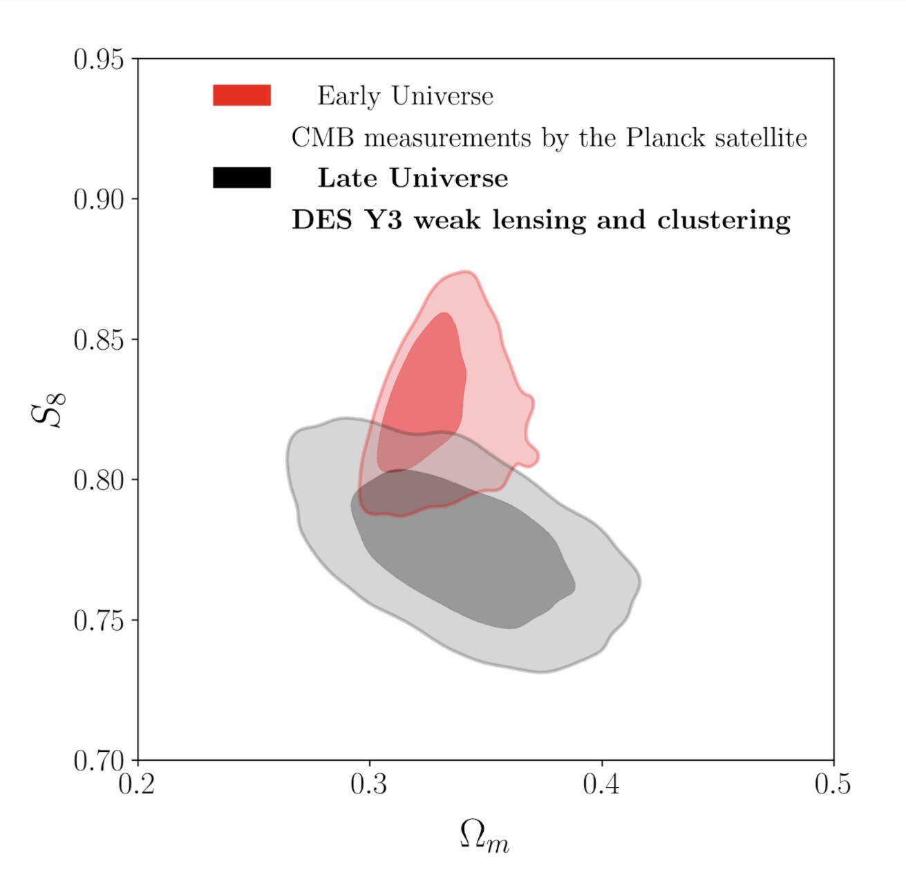
Figure 3: A plot showing constraints on the average matter density of the Universe (Ω_m), and the size of density fluctuations (S_8) from late-Universe DES measurements (gray) and early-Universe CMB measurements (red). Tension between the early and late Universe measurements can be seen as an offset between these two sets of contours. (Credit: DES Collaboration.)
Figure 3 shows a main result of the DES Year 3 analysis: constraints on the two cosmological parameters that DES constrains the best—the matter density Ωm, and the amplitude of density fluctuations quantified by S8. The gray contours show parameter estimates based on DES measurements, and the red contours show estimates based on Planck satellite measurements of the Cosmic Microwave Background (CMB). In both cases, the darker inner contour identifies the region where our posterior estimate tells us the real values of the parameters have a 68% chance of being found. The outer lighter gray contour shows the 95% confidence region.
CMB measurements are sensitive mainly to the properties of the early Universe, about 300,000 years after the Big Bang. Effectively, the Planck (red) S8 contours tell us the amplitude of density fluctuations we expect to see today, based on measurements of the early Universe and assuming our model for how density fluctuations evolve over time. The gray DES contours show more direct measurements of the distribution of matter in the late-Universe. Thus, comparing DES and Planck constraints on S8 is a powerful test of how well our cosmological model can describe the evolution of structure over 13 billion years of cosmic history. A mismatch between those constraints could be a hint that we need to include additional physics in our model.
In the plot we see that DES constraints prefer a lower value of S8 than Planck (similar to the discrepancy previously found in the analysis of the first year of DES data, reported by the DES Collaboration in 2017). In other words, the amount of structure we see in the late Universe is slightly less than we’d expect given the early-Universe CMB measurements and our standard cosmological model. Statistically speaking, this offset is not large enough to be considered significant but—tantalizingly—the direction of the offset is similar to that found by other independent weak lensing surveys like the Kilo-Degree Survey and the Hyper Suprime Cam survey. The agreement of several different late-Universe measurements suggest that there may yet be something interesting to learn, as we combine and compare different weak lensing measurements (as in this paper) and gather more precise data in the future.
We’re also investigating what these data have to say about cosmological models which add new physics to our description of the Universe. Results using DES Y3 galaxy clustering and weak lensing measurements to constrain more cosmological models will be featured in an upcoming darchive! (This is what I mainly work on.)
We’ll be watching the S8 comparison and other tests of our cosmological model closely as we analyze the full six-year DES dataset—as well as the data promised by the next-generation Rubin Observatory Legacy Survey of Space and Time, to begin soon at the Vera Rubin Observatory on the next mountaintop over from our own Blanco telescope.
We’ve accomplished a lot in the DES Year 3 analyses, but we still have further to go. The assessment from 2017 holds:
“Work remains. More exploration must be done.”
DArchive Author: Jessie Muir
 Jessie is a postdoctoral fellow at the Perimeter Institute for Theoretical Physics in Waterloo, Ontario. Within DES she works on theory and the combined analysis of multiple cosmological observables. She co-led the analysis team behind the collaboration’s recently released Year 3 galaxy clustering and weak lensing study constraining physics beyond the standard cosmological model, and also contributed to the development of the methods DES uses to protect its analysis from unconscious experimenter bias. In her spare time, she enjoys drawing (including several of the #darkbites cartoons illustrating DES Y3 papers!), cooking, reading, yoga, and texting friends an excessive number of cat photos.